Random variables
A random variable is a numerical representation of a random event.
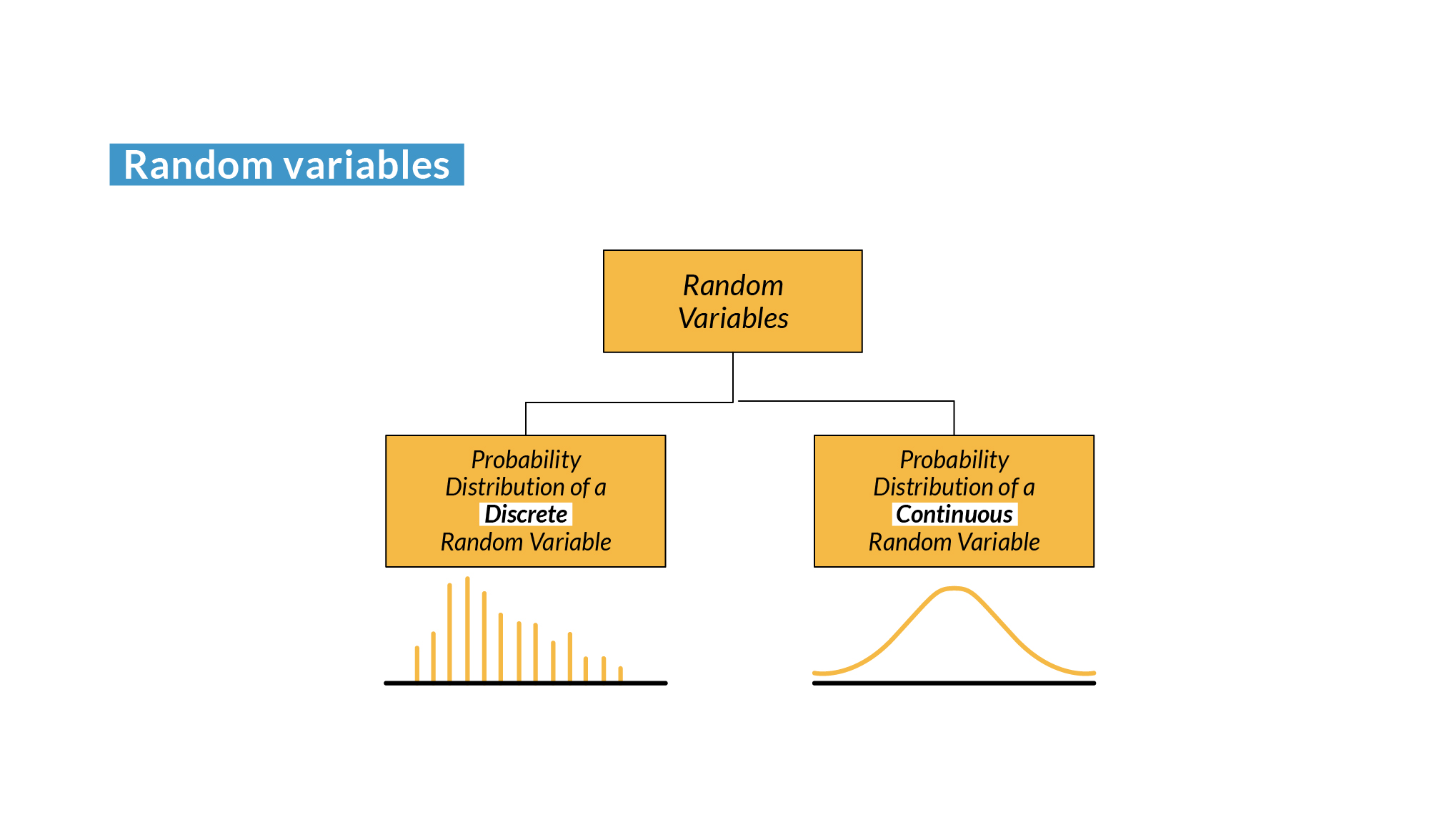
Types of random variables
Due to the nature of random events, they can be discrete or continuous.
- Discrete random variable: Can take a countable, finite number of distinct values. For example, the number of times heads comes up when flipping a coin 10 times is a discrete random variable, since it can have values such as 0, 1, 2, ..., 10.
- Continuous random variable: It can take any value in a continuous interval. For example, the height of a randomly selected person is a continuous random variable because it can be any value within a reasonable range, such as between 50 cm and 250 cm.
Each random variable has an associated distribution function, which describes the probability that the random variable will take a specific value (for discrete variables) or fall within a specific interval (for continuous variables).
Distribution functions
In statistics, we represent a distribution of discrete variables through probability mass functions (PMF). The PMF defines the probability of all possible values of the random variable. In random variables, we represent their distribution by means of the probability density function (PDF).
Probability mass function
It is specific to discrete random variables and gives the probability that the random variable will take a particular value.
import matplotlib.pyplot as plt
import numpy as np

data = np.arange(1, 7)
pmf = [1/6 for _ in data]

plt.figure(figsize = (10, 5))
plt.stem(data, pmf)
plt.title("PMF - Roll a die")
plt.xlabel("Die value")
plt.ylabel("Probability")
plt.xticks(data)
plt.show()

In this case, we see that the distribution of the random variable is uniform, since its probabilities do not change.
Probability density function
It is specific for continuous random variables, and it's the same as the PMF, but for continuous variables.
from scipy.stats import norm

data = np.linspace(-5, 5, 1000)
pdf = norm.pdf(data)

plt.figure(figsize = (10, 5))
plt.plot(data, pdf, "r-")
plt.title("PDF - Normal distribution")
plt.xlabel("Value")
plt.ylabel("Density")
plt.show()

In this case, we see that the distribution is normal, since the graph faithfully reproduces a Gaussian bell.
Cumulative distribution function
A cumulative distribution function (CDF) is defined for discrete and continuous variables and measures the probability that the random variable takes a value less than or equal to a given one.
data = np.linspace(-5, 5, 1000)
cdf = norm.cdf(data)

plt.figure(figsize = (10, 5))
plt.plot(data, cdf, "r-")
plt.title("CDF - Normal distribution")
plt.xlabel("Value")
plt.ylabel("Probability")
plt.show()

If we relate the two previous functions:
data = np.linspace(-5, 5, 1000)
pdf = norm.pdf(data)
cdf = norm.cdf(data)

plt.figure(figsize = (10, 5))
plt.plot(data, pdf, "r-")
plt.plot(data, cdf, "b-")
plt.xlabel("Value")
plt.show()

Probability distributions
Probability distributions describe how the probabilities of a random variable are distributed. There are many probability distributions, and each describes a different type of random process.
Binomial distribution
The binomial distribution applies to discrete random variables and describes the number of successes in a set of independent Bernoulli experiments. These experiments must have two possible outcomes. For example, the number of heads obtained by tossing a coin 10 times.
from scipy.stats import binom

n_experiments = 100
probability = 0.5

data = range(n_experiments)
pmf = binom.pmf(data, n_experiments, probability)

plt.figure(figsize = (10, 5))
plt.stem(data, pmf)
plt.show()

Poisson distribution
The Poisson distribution applies to discrete random variables and describes the number of events that occur in a fixed interval of time or space, given an average rate of occurrence. For example, the number of calls received by a call center in an hour.
from scipy.stats import poisson

n_experiments = 10
n_occur = 5

data = range(n_occur * n_experiments)
pmf = poisson.pmf(data, n_occur)

plt.figure(figsize = (10, 5))
plt.stem(data, pmf)
plt.show()

Geometric distribution
The geometric distribution applies to discrete random variables and measures the number of trials required to obtain the first success in independent Bernoulli experiments. For example, the number of coin tosses needed to obtain the first head.
from scipy.stats import geom

n_experiments = 25
probability = 0.5

data = range(1, n_experiments)
pmf = geom.pmf(data, probability)

plt.figure(figsize = (10, 5))
plt.stem(data, pmf)
plt.show()

Normal distribution
The normal distribution applies to continuous random variables and is bell-shaped; hence, it is also called Gaussian distribution. It is determined by two parameters: the mean $mu$ and the standard deviation $sigma$. For example, the distribution of heights or weights in a large population.
from scipy.stats import norm

mu, sigma = 0, 1

data = np.linspace(-5, 5, 1000)
pdf = norm.pdf(data, mu, sigma)

plt.figure(figsize = (10, 5))
plt.plot(data, pdf)
plt.show()

Exponential distribution
The exponential distribution applies to continuous random variables and describes the time between events in a Poisson process. For example, the time until an electronic device fails. It is the continuous counterpart of the geometric distribution.
from scipy.stats import expon

data = np.linspace(0, 5, 1000)
pdf = expon.pdf(data)

plt.figure(figsize = (10, 5))
plt.plot(data, pdf)
plt.show()

Uniform distribution
The uniform distribution applies to continuous random variables and assumes that all values in an interval have the same probability of occurrence. For example, select a random number between 0 and 1.
from scipy.stats import uniform

data = np.linspace(-2, 2, 1000)
pdf = uniform.pdf(data, loc = -1, scale = 2)

plt.figure(figsize = (10, 5))
plt.plot(data, pdf)
plt.show()

Chi-square distribution
The Chi-square distribution applies to continuous random variables and is widely used for hypothesis testing and contingency tables.
from scipy.stats import chi2

df = 5
data = np.linspace(0, 20, 1000)
pdf = chi2.pdf(data, df)

plt.figure(figsize = (10, 5))
plt.plot(data, pdf)
plt.show()

Student's t distribution
The Student's t distribution applies to continuous random variables and is similar to the normal distribution but with heavier tails. It is useful when the population size is small.
from scipy.stats import t

data = np.linspace(-10, 10, 100)
pdf = t.pdf(data, df)

plt.figure(figsize = (10, 5))
plt.plot(data, pdf)
plt.show()

Each of these distributions has its own set of parameters and associated formulas. The choice of distribution depends on the nature of the experiment or process being modeled.