How to deal with missing values
Why do we need to fill in missing values?
Because most of the machine learning models that we want to use will provide an error if we pass NaN values into it. However, algorithms like K-nearest and Naive Bayes support data with missing values. The easiest way is to fill them up with 0 but this can reduce our model accuracy significantly.
Before we start deleting or imputing missing values, we need to understand the data in order to choose the best method to treat missing values. You may end up building a biased machine learning model which will lead to incorrect results if the missing values are not handled properly.
As we saw in the exploratory data analysis, we can find missing values by using the info() function and looking at how many non-null values are in each column. Another way is using isnull() function.
Types of missing values
1. Missing completely at random
Missing values are completely independent of other data. There is no pattern. For Example, suppose in a library there are some overdue books. Some values of overdue books in the computer system are missing. The reason might be a human error like the librarian forgot to type in the values. So, the missing values of overdue books are not related to any other variable/data in the system.
It should not be assumed as it’s a rare case. The advantage of such data is that the statistical analysis remains unbiased.
2. Missing at random
The reason for missing values can be explained by variables on which you have complete information as there is some relationship between the missing data and other values/data. It is missing only within sub-samples of the data and there is some pattern in the missing values.
For example, in a survey, you may find that all the people have answered their ‘Gender’ but ‘Age’ values are mostly missing for people who have answered their ‘Gender’ as ‘female’. (The reason being most of the females don’t want to reveal their age.)
So, the probability of data being missing depends only on the observed data.
Suppose a poll is taken for overdue books of a library. Gender and the number of overdue books are asked in the poll. Assume that most of the females answer the poll and men are less likely to answer. So why the data is missing can be explained by another factor that is gender.
In this case, the statistical analysis might result in bias.
3. Missing Not At Random
Missing values depend on the unobserved data. If there is some pattern in missing data and other observed data can not explain it, then it is Missing Not At Random.
It can happen due to the reluctance of people in providing the required information. A specific group of people may not answer some questions in a survey. For example, people with more overdue books are less likely to answer the poll about number of overdue books. Another example would be people having less income may refuse to share that information in a survey. The statistical analysis might result in bias.
Methods to deal with missing values
1. Deleting the column that has missing values
It should only be used when there are many null values in the column. We can do this by using dataframe.dropna(axis=1) or by using drop() and specifying the column we want to drop. The problem with this method is that we may lose valuable information on that feature, as we have deleted it completely due to some null values. Since we are working with both training and validation sets, we are careful to drop the same columns in both DataFrames.
#Code to drop a certain column
df2 = df.drop(['column_to_drop'],axis=1)
2. Deleting rows that have missing values
We can delete only the rows that have missing values by using the dropna() function again. This time we will use axis=0 as parameter because instead of looking for columns with missing values, we are looking for rows with missing values.
If a row has many missing values then you can choose to drop the entire row. If every row has some (column) value missing then you might end up deleting the whole data.
#Dropping all rows that have any null value
df2 = df.dropna(axis=0)
We can add a 'threshold' to our function. That way dropping rows will meet the threshold conditions first. For example if we write the following function :
#It will keep the rows with at least 2 non-NA values.
df2=df.dropna (axis = 0, thresh=2)
This can be used in percentages too.
#It will drop all rows with null values except the ones that have at least 65% of data filled (non null values).
df2=df.dropna (axis = 0, thresh= 0.65 * len(df))
Threshold can be used in rows, as well as columns using axis= 1.
3. Filling missing values - Imputation
In this method we fill null values with a certain value. Although it's simple, filling in the mean value generally performs quite well. While statisticians have experimented with more complex ways to determine imputed values (such as regression imputation, for instance), the complex strategies typically give no additional benefit once you plug the results into sophisticated machine learning models. There are some ways to impute missing values:
- Mean imputation
If it is a numerical feature, we can replace the missing values with the mean, but make sure the specific feature does not have extreme values so that the mean can still represent a central tendency.
Example:
#Replacing a column null values with the column mean
df['column_to_impute'] = df['column_to_impute'].fillna(df['column_to_impute'].mean())

#Imputing null values using scikit learn SimpleImputer
from sklearn.impute import SimpleImputer
my_imputer = SimpleImputer(strategy = 'mean')
new_df = my_imputer.fit_transform(df)
- Median
If it is a numerical feature and the feature has extreme values, which we had decided to keep, then those outliers will pull the mean towards the extremes and it will not represent a central tendency anymore. In that case, we should consider using the median instead.
Example:
df.fillna(df.median())

#Imputing null values using scikit learn SimpleImputer

from sklearn.impute import SimpleImputer
my_imputer = SimpleImputer(strategy = 'median')
new_df = my_imputer.fit_transform(df)
- Mode
Another technique is mode imputation in which the missing values are replaced with the mode value or most frequent value of the entire feature column. When the data is skewed, it is good to consider using mode values for replacing the missing values. For data points such as the Embarked field, you may consider using mode for replacing the values. Note that imputing missing data with mode values can be done with numerical and categorical data.
Example:
df['column_to_impute'] = df['column_to_impute'].fillna(df['column_to_impute'].mode()[0])

#Imputing null values with scikit learn SimpleImputer

from sklearn.impute import SimpleImputer
imputer = SimpleImputer(strategy='most_frequent')
imputer.fit_transform(X)
-Create a new category for categorical features
Impute the Value “missing”, which treats it as a Separate Category to replace null values in a categorical feature.
Example:
#Creating a new category named 'missing' to replace null values
imputer = SimpleImputer(strategy='constant', fill_value='missing')
imputer.fit_transform(X)
- New Value
Filling the numerical value with 0 or -999, or some other number that will not occur in the data. This can be done so that the machine can recognize that the data is not real or is different.
Example:
#Replace the missing value with '0' using 'fiilna' method
df['column_to_impute'] = df['column_to_impute'].fillna(0)
- Other imputation methods
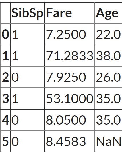
In a multivariate approach, more than one feature is taken into consideration. There are two ways to impute missing values considering the multivariate approach. Using KNNImputer or IterativeImputer classes. To explain them, we will do assumptions using the Titanic example.

- Iterative imputation
Suppose the feature ‘age’ is well correlated with the feature ‘Fare’ such that people with lower fares are also younger and people with higher fares are also older.
In that case, it would make sense to impute low age for low fare values and high age for high fares values. So here we are taking multiple features into account by following a multivariate approach.
cols = ['SibSp', 'Fare', 'Age']
X = df[cols]

from sklearn.experimental import enable_iterative_imputer
from sklearn.impute import IterativeImputer
impute_it = IterativeImputer()
impute_it.fit_transform(X)
In this case, the null values in one column are filled by fitting a regression model using other columns in the dataset. For all rows, in which ‘Age’ is not missing scikit learn runs a regression model. It uses ‘Sib sp’ and ‘Fare’ as the features and ‘Age’ as the target. And then for all rows for which ‘Age’ is missing, it makes predictions for ‘Age’ by passing ‘Sib sp’ and ‘Fare’ to the training model. So it actually builds a regression model with two features and one target and then makes predictions on any places where there are missing values. And those predictions are the imputed values.
- Nearest Neighbors Imputations (KNNImputer)
Missing values are imputed using the k-Nearest Neighbors approach where a Euclidean distance is used to find the nearest neighbors.
cols = ['SibSp', 'Fare', 'Age']
X = df[cols]

from sklearn.impute import KNNImputer
impute_knn = KNNImputer(n_neighbors=2)
impute_knn.fit_transform(X)
Let's look at the data again:

As the n_neighbors = 2, scikit learn finds the two most similar rows measured by how close the ‘Sib sp’ and ‘Fare’ values are to the row which has missing values. In this case, the last row has a missing value. And the third row and the fifth row have the closest values for the other two features. So the average of the ‘Age’ feature from these two rows is taken as the imputed value.